Python is notorious for coming with batteries included. This is a humorous way of saying that the Python standard library is fairly extensive, and its capabilities are not limited to the bare minimum you would expect from a casual programming language. We have covered that in Chapter 2.
Python is also, by its very own nature, a general-purpose programming language and, while the standard library allows you to send emails, or parsing all the most widely used text formats out there, it is not necessarily the best place to start if you crunch numbers as a day job. As a physicist and/or data scientist, you will need to dive into the Python scientific stack.
The Python scientific ecosystem is a thriving environment, with lots of interesting things happening every day—definitely something to stay tuned on. We shall only cover (and superficially, too) the classical packages:
NumPy: a numerical library offering a powerful n-dimensional array type, along with an extensive set of mathematical functions and facilities that inter-operate natively with it;
SciPy: the fundamental scientific package, building on top of NumPy and providing facilities for integration, optimization (aka fitting), interpolation, signal processing;
matplotlib: the standard package for visualization and plotting in Python;
pandas: a popular, high-level analysis tool—a must if you happen to work with excel files.
All of the above are sponsored by the NumFocus initiative, and you should take a look at the long list of supported packages: chances are that you will find something tha fits you.
6.1 NumPy
The fundamental package for scientific computing with Python.
At the very fundamental level, NumPy offers a new Python data type—a n-dimensional array:
import numpy as npa = np.array([1., 2., 3.])m = np.array([[1, 0], [0, 1]])for item in a, m:print(item)print(f"Data type: {item.dtype}, shape: {item.shape}")
[1. 2. 3.]
Data type: float64, shape: (3,)
[[1 0]
 [0 1]]
Data type: int64, shape: (2, 2)
There is a number of convenient ways you can initialize a NumPy array, other that manually from Python iterables:
Commit all of them to memory if you haven’t done it already, because you will put each single one of them to good use, sooner or later. More details on the documentation page about array creation.
6.1.1 Array and native Python types
Before we dig into the gory details of how you can use NumPy arrays in your daily workflow, it is useful to clarify some of the main differences with respect to the native Python data types.
When looked at superficially, NumPy arrays look a lot like Python lists:
Sure enough, they are both iterables, but that’s pretty much it. For one thing Python lists are heterogeneous, while NumPy arrays are intrinsically homogeneous (more about types in a second). The semantic of the support that they offer to elementary arithmetic is completely different:
import numpy as npl = [1, 2, 3]a = np.array([1, 2, 3])print(f"sum: {l + l} vs. {a + a}")print(f"multiplication by a scalar: {l *2} vs. {a *2}")
sum: [1, 2, 3, 1, 2, 3] vs. [2 4 6]
multiplication by a scalar: [1, 2, 3, 1, 2, 3] vs. [2 4 6]
That is: for native Python lists sum means concatenation and multiplication by a scalar means simply repetition; in the case of NumPy arrays both operations are intended as element by element. Stop for a second and think about what is the most useful semantic for data analysis.
There are other notable differences, some of which we shall discuss in more details in the following of this chapter. Python lists and arrays have a completely different layout (and footprint) in memory and, as we shall see, they do operate at a fundamentally different speed. Arrays offer a much more powerful indexing and slicing. Arrays inter-operate natively with the NumPy and SciPy mathematical functions.
But, before we move on and look into all of this, there is another odd corner that is worth pointing out—especially for those of you who learned (or are learning) Python as their first language. NumPy arrays always come with in a specific type—we know this already:
As you might notice, no matter how you specify the data type, since at the fundamental level NumPy is largely implemented in C, it is the underlying C data types that it uses—not Python’s. (Suggested reading.) Now, for floating point numbers this does not make a whole lot of difference, but when you do operate on arrays of integers the consequences are dramatic, as you immediately loose the luxury of infinite-precision integer arithmetic that you are so used to:
import numpy as npa = np.array([2, 4, 8, 16])print(a.dtype)print(a**16)
int64
[          65536      4294967296 281474976710656               0]
Make sure you understand this before you move on: you see the last zero in the output? The fact is: NumPy is storing the elements of out arrays as (signed) 64-bit integers, which means that the maximum value they can hold before overflow occurs is \[
2^{63} - 1 = 9223372036854775807
\] whereas the value we are trying to represent is too large: \[
16^{16} = (2^4)^{16} = 2^{64} = 18446744073709551616.
\]
This happens in real life. Really. You are advised. 🔥
6.1.2 Indexing and slicing
This is covered in details here. To first approximation, indexing works just as it does in ordinary Python lists, that is
import numpy as npl = [1, 2, 3]a = np.array(l)print(l[0])print(a[0])
1
1
Working with multidimensional arrays is fairly intuitive once you commit to memory that NumPy uses C-order indexing, which means that the last index represents the most rapidly changing memory location. For 2-dimensional arrays (i.e., ordinary matrices, or rank-2 tensors) this means that the first index indicates the rows, while the second runs over the columns:
A boolean array used for the purpose of indexing another array is customarily called a mask. As we shall see in a second, this is important when vectorizing problems, as this trick allows to emulate what we would achieve with conditional statements in a normal loop.
As we said, all the gory details are in the documentation page about indexing, and it doesn’t make sense to repeat everything here.
6.1.3 Broadcasting
This is covered in details here. As we said, arithmetic operations on NumPy arrays are generally to be intended as element-wise, that is
import numpy as npa = np.array([1., 2., 3.])b = np.array([4., 5., 6.])print(a + b)print(a * b)
[5. 7. 9.]
[ 4. 10. 18.]
Interestingly, arithmetic operations in NumPy are not limited to arrays with the same exact shape. Look at the following examples:
This behavior goes under the name of broadcasting. NumPy broadcasting rules are explained here and we will not overlap with that. In the simplest cases the thing is fairly intuitive, but you should take your time to master it, because broadcasting is central to vectorization, as we shall see in the next section.
Before we move on, though, it is worth mentioning that this very basic idea of element-wise operations is not limited to elementary arithmetic, and covers all the mathematical functions defined in NumPy and derived scientific packages:
import numpy as npa = np.linspace(0.1, 1., 10)print(a)print(np.log10(a))print(np.exp(a))print(np.sin(a))
Make sure you fully understand that, io order for this to work, you really need mathematical functions that are designed for the purpose—the Python standard library is not helping, here
import mathimport numpy as npa = np.linspace(0.1, 1., 10)print(math.log10(a))
---------------------------------------------------------------------------TypeError Traceback (most recent call last)
CellIn[14], line 7 3importnumpyasnp 5 a = np.linspace(0.1, 1., 10)
----> 7print(math.log10(a))
TypeError: only length-1 arrays can be converted to Python scalars
But don’t worry: if you need mathematical functions, SciPy has your back.
6.1.4 Vectorization
If there is one thing that Python is not famous for, that is speed. Quite the contrary, Python has a fairly consolidated name for being slooooow.
On the face of it, you shouldn’t be surprised. We have been bragging all along about all the nice features that Python offers—the fact that you don’t have to declare variables, or that containers can be heterogeneous, infinite-precision integer arithmetic, you name it. Since, as Richard Feynman used to say, there is no free lunch in quantum electrodynamics, all these good things come at a price. And the price, in this case, is called speed.
Do I really care, you ask? Well, it depends. If you are parsing a text file or fetching a web page, probably not. If a task takes 2 ms to complete, and you are not doing it 1000 times a second, beating down the execution time by a factor of ten wouldn’t really make a difference. As a human, all you notice is that you press enter and you are immediately done in both cases.
If, on the other hand, you are performing a CPU-intensive processing on a TB of data, then probably yes—speed matters. If you can beat down the execution time from 20 minutes to 10 seconds, that is a game changer—you don’t have to go have a coffee in between two consecutive runs, and since too much coffee is bad for you, that is a net positive. Also, you have a much shorter development cycle, which will help you in the long run.
(Before you move one, make sure you have fully digested both paragraphs above. You don’t need to optimize everything. So much so that the saying goes: premature optimization is the root of all evil. We shall get back to that in Chapter 11.)
Fortunately, when you do need to optimize, NumPy is one of the things that might come to rescue. Why is that? Well, NumPy is written in C as a Python extension, and the underlying functions are highly optimized to crunch numbers. In other words, when you perform array operations using NumPy, you are actually executing optimized C code. How cool is that?
Let’s see that in action. As you probably know, every programming language comes with a pseudo random number generator (PRNG), which is the physicist’s best friend when it comes to setup simulations. (PRNGs typically generate numbers equi-distributed between 0 and 1, and then there are well-defined techniques to transform them into arbitrary distributions.) Python is no exception, as the standard library provides the random module; on top of that, NumPy offers its own PRNG.
Which one shall we use? Well, let us assume we want to generate 1 million random numbers, and let’s check out both!
import randomimport timeimport numpy as npn =1000000# The slow way: explicit for loop in Python.t0 = time.time()x = []for i inrange(n): x.append(random.random())dt = time.time() - t0print("Elapsed time: %.4f s"% dt)# The quick way: using numpy.t0 = time.time()x = np.random.random(size=n)dt = time.time() - t0print("Elapsed time: %.4f s"% dt)
Elapsed time: 0.0659 s
Elapsed time: 0.0084 s
Note
Note the two block of code are (roughly) equivalent from a functional point of view, but surely not on a number by number basis. For one thing the pure-Python version creates a list of random numbers, while the NumPy version creates an array (of the same length). That said, Python uses the Mersenne Twister as the core generator, while NumPy uses by default PCG-64, a 128-bit implementation of O’Neill’s permutation congruential generator. And, even if they used the same underlying algorithm, you would have to set the seed explicitly to get the same sequence. None of this is really relevant to the point we are trying to make.
All right. The main take-away message here is: NumPy generates the same amount of random numbers as plain Python in about a tenth of the time—not bad. Let’s be very explicit: the fact that in Python you need a for loop (lines 9–11) while the rough NumPy equivalent is a one-liner (line 17) does not mean that there is no loop in the second version. The loop is implicit and, as we said, it happens at the speed of C. Much faster than Python.
Which immediately brings to the corollary: avoid for loops in pure Python when crunching numbers. It’s ok to use a for loop if you have to iterate over the lines of a small text file, of the files in a folder on your machine. Not so much over millions and millions of numbers. You get the difference.
Let us push this a little bit farther in the context of a toy Monte Carlo simulation of a gas detector. More specifically, let’s say we have a beam of \(E_0 = 6\) keV monochromatic X-rays impinging on a gas cell where the average energy necessary to create an electron-ion pair by ionization is \(W_i = 30\) eV. Every time a photon undergoes photoelectric absorption, a photoelectron is emitted, and the latter ionizes the gas creating \(E_0 / W_i = 200\) primary electrons on average (we shall assume this is Poisson distributed), each of which is in turn multiplied through a avalanche-like process with a mean gain \(G = 100\), with an underlying exponential distribution. The total number of ionization pairs is our measure of the energy, and we are interested in measuring the energy resolution of the detector. (Note this is the sum of 200 exponential random variables which, by virtue of the central limit theorem, is approximately gaussian distributed. I will leave it to you to calculate the expected mean and variance.)
Note
A little piece of advice before we actually move forward with our plan. If you happen to do real work on gas detectors, be advised we are making at least to big mistakes as far as the underlying physics goes, here. For one thing, the primary ionization is not Poisson distributed—the phenomenon is under-dispersed and the corresponding variance is smaller than what you would expect based on the Poisson distribution by a factor \(F\) called the Fano Factor. Additionally, in a realistic gas detector, the gain distribution is more complex than an exponential, and is often parametrized as a Polya function. But this is all about explaining vectorization, not doing real simulations.
How would we go about simulating this process in Python? Well, here is something that might do the trick:
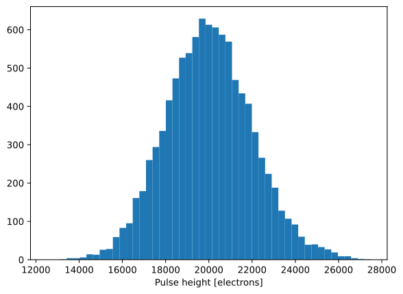
import randomimport timeimport numpy as npfrom matplotlib import pyplot as pltnum_photons =10000E_0 =6000.# eVW_i =30.# eVG =100.pha = []t0 = time.time()# Outer loop over the impinging X-rays.for i inrange(num_photons):# Initialize the total number of the electron-ion pairs that are created# by ionization for this particular event. total_ionization =0# Extract the number of primary electrons created by the photoelectron.# Too bad the random module in the standard lib does not provide the# Poisson distribution, and we do have to resort to numpy... num_primaries = np.random.poisson(E_0 / W_i)# Inner loop over the primary electrons...for j inrange(num_primaries):# For each primary electron, extract the number of electron-ion pairs# generated in the avalanche. total_ionization += random.expovariate(1./ G) pha.append(total_ionization)dt = time.time() - t0plt.hist(pha, bins=np.linspace(12500., 27500., 50))plt.xlabel("Pulse height [electrons]")print(f"Simulation completed in {dt:.3f} s")
Simulation completed in 0.293 s
Now, can I speed things up using NumPy? You bet you can!
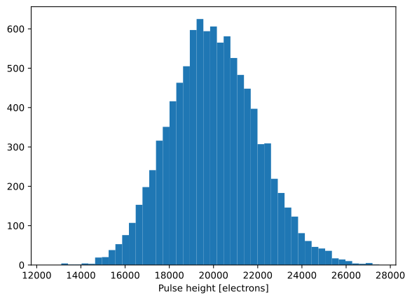
import timeimport numpy as npfrom matplotlib import pyplot as pltrng = np.random.default_rng()num_photons =10000E_0 =6000.# eVW_i =30.# eVG =100.t0 = time.time()# Create an array with the number of primaries for each single X-ray.num_primaries = rng.poisson(E_0 / W_i, size=num_photons)# Populate an array with as many copies of the event id as the corresponding# primary electronsevent_id = np.repeat(np.arange(num_photons), num_primaries)# Extract the gain for each single primary electron.event_gain = rng.exponential(scale=G, size=event_id.size)# Sum all the ionization pairs, on an event-by-event basis, to get the "energy".pha = np.bincount(event_id, weights=event_gain, minlength=num_photons)dt = time.time() - t0plt.hist(pha, bins=np.linspace(12500., 27500., 50))plt.xlabel("Pulse height [electrons]")print(f"Simulation completed in {dt:.3f} s")
Simulation completed in 0.014 s
Let’s take a breath. The histograms look similar to each other, which is good. (As I said: I will leave it to you to asses whether the mean and the standard deviations look reasonable, based on our initial assumptions.) The numpy version is roughly a factor of 20 faster—this is also good news.
But the one thing you should be really be paying attention to is the fundamentally different way the problem is cast in the two cases. In the pure-Python version we have an outer loop over the events, and we process each one before we move to the next; in the second version we perform each physical step of the simulation (i.e., extract the number of primary electrons, extract the avalanche size) for all the events at the same time.
This latter approach is sometimes called vectorization, and you readily see the pros and the cons. The pure-Python version is easier to read, as it proceeds in the same temporal order that it would in real life. In the vectorized version we are mixing things up—in this particular case first comes the primary ionization for all the X-rays, then the avalanche for all the primary electrons. The flow is not nearly as natural to follow, and it also implies a larger memory footprint, because we have to keep track of larger arrays. The advantage: we can delegate all the (now implicit) loops to NumPy and they happen at the speed of C.
Vectorization with NumPy is a difficult language to learn. At the very fundamental level the basic rules are:
all the loops are implicit, and you keep everything in memory;
conditional branches in the control flow are achieved via masks;
in many cases you have to resort to (more or less) obscure NumPy functions such as bincount to achieve what you need.
Mastering this language is one of the avenues to be able to do a sensible simulation in Python.
6.2 SciPy
Fundamental algorithms for scientific computing in Python .
We are going very fast on this one. Among the various things that SciPy has to offer we list:
Splines are interesting objects, and not nearly as widely known as they deserve, which is why we are taking a small detour, here. (When we have a series of point, we physicist have a tendency to insist fitting a function through them, where in some cases interpolating is really the right thing to do.)
Technically speaking, splines are functions passing through a series of given points, defined piecewise by polynomials of fixes degree \(k\). (\(k = 3\) is a fairly popular choice, but values between 1 and 5 are used.)
If you think about for a second, for \(n\) point you have \(kn\) parameters, which gives you enough freedom to:
have the spline pass exactly through every point;
have the first \(k - 1\) derivatives continuous everywhere.
All the coefficients of the polynomials are calculated once and forever at creation time, based on the coordinates of the control points.
Making a spline using SciPy is as easy as
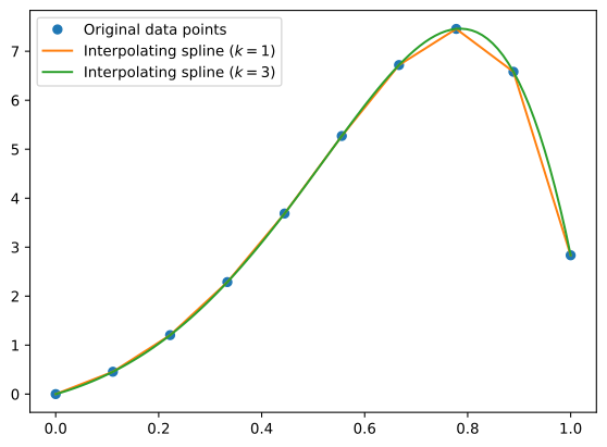
import numpy as npfrom scipy.interpolate import InterpolatedUnivariateSplinex = np.linspace(0., 1., 10)y = np.exp(3.* x) * np.sin(3.* x)s1 = InterpolatedUnivariateSpline(x, y, k=1)s3 = InterpolatedUnivariateSpline(x, y, k=3)xgrid = np.linspace(0., 1., 100)plt.plot(x, y, "o", label="Original data points")plt.plot(xgrid, s1(xgrid), label="Interpolating spline ($k = 1$)")plt.plot(xgrid, s3(xgrid), label="Interpolating spline ($k = 3$)")plt.legend()
For \(k = 1\) you get a broken line, whose first derivatives are discountinuous at the control points; for \(k = 3\) you get a so-called cubic spline, which is well behaved in most situations. If all you care is literally getting a smooth curve that goes through a series of point, with no underlying physics or insight, splines are often superior to polynomial interpolation or curve fitting.
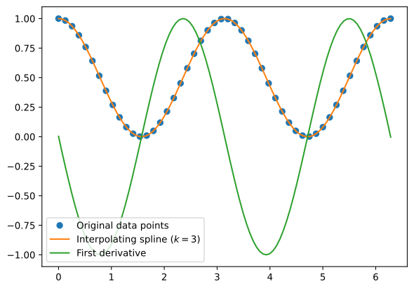
There is a few more extra goodies that you get for free when you buy into splines. Evaluation is fairly inexpensive: all you need to do is find the two control points that include the \(x\) value where you want to evaluate, and since the input array of \(x\) coordinates is required to be sorted, this can be done via a binary search with a complexity \(O(\log n)\). In addition, since this is all as simple al polynomials, derivatives and integrals are easy:
import numpy as npfrom scipy.interpolate import InterpolatedUnivariateSplinex = np.linspace(0., 2.* np.pi, 50)y = np.cos(x)**2s = InterpolatedUnivariateSpline(x, y, k=3)xgrid = np.linspace(0., 2.* np.pi, 100)plt.plot(x, y, "o", label="Original data points")plt.plot(xgrid, s(xgrid), label="Interpolating spline ($k = 3$)")plt.plot(xgrid, s(xgrid, 1), label="First derivative")plt.legend()print(s.integral(0., 2.* np.pi)) # <- this should be approximately pi
3.1416006818156785
Really: take a few minutes to dive into spline, because they might come a time in your life when they are the right tool to use.
6.3 pandas
A fast, powerful, flexible and easy to use open source data analysis and manipulation tool.
And we are at the end of the chapter. Not before we mention pandas, though.
Chances are that, sooner or later, you will have to deal with spreadsheets for a particular task. (It might be an administrative task, as opposed to one related to pure research, but keep in mind these will come too.) When that happen, pandas read_excel() function is there for you. Basic usage is as simple as
import pandas as pddf = pd.read_excel("data.xlsx")
We don’t have time to drag this any longer, but pandas is definitely another keyword that you want to commit to memory and have it at hand in case of need.