def gcd(n: int, m: int) -> int:
    r = n % m
    while r != 0:
        n = m
        m = r
        r = n % m
    return m

print(gcd(49, 21))7Algorithm: (noun) a list of instructions for solving a problem. Source: the Cambridge Dictionary, again.
Easy, isn’t it? Here is one of the most popular words of the last decade, demystified. In this chapter we shall glance (and fairly quickly, too) through two very important and inter-related topics: algorithms and data structures. Using the right algorithm and/or data structure sometimes makes all the difference between being able to attack a problem in a practical time or not, so pay attention.
If there is a classic algorithm that has passed the test of time, it is that due to Euclid to find the greatest common divisor (GCD) between two integers, so this is where we shall start from. Keep in mind, algorithms can be expressed in several different ways: flow-charts, pseudo-code, working code snippets—you name it. The main point is that the sequence of operation must be expressed unambiguously.
Let \(n\) and \(m\) be two positive integers. The following procedure will converge to the GCD between the two in a finite number of steps:
(Here \(n \leftarrow m\) means simply: replace \(n\) with the value of \(m\).)
This is not a course in number theory, so we shall refrain from demonstrating that what we just said is actually true. Lazy as we are, we will just go ahead, implement the thing in Python and observe it in action.
def gcd(n: int, m: int) -> int:
r = n % m
while r != 0:
n = m
m = r
r = n % m
return m
print(gcd(49, 21))7Well, \(49 = 7 \times 7\) and \(21 = 7 \times 3\), so the answer is correct. In this particular case the algorithm completes in two iteration, and it is instructive to write down the values of all the relevant variables at each step.
| Iteration | \(n\) | \(m\) | \(r\) |
|---|---|---|---|
| 1 | \(49\) | \(21\) | \(7\) |
| 2 | \(21\) | \(7\) | \(0\) |
You see what’s happening and why the thing works: at each step we are dealing with pairs of numbers that are smaller and smaller, until the remainder of the division becomes zero and we are done.
It is somewhat amusing to note that, had we started with \(n = 21\) and \(m = 49\) the first step of the algorithm would have simply swapped the two numbers, and we would have reached the same result, although with the need of one extra iteration.
Think about it. How many iteration does it take for the Euclidean algorithm to converge? Well, this is an ill-posed question. I mean: give me two integers and I can have my program count the number of steps it take
def gcd_iterations(n: int, m: int) -> int:
    r = n % m
    k = 1
    while r != 0:
        n = m
        m = r
        r = n % m
        k += 1
    return k

print(gcd_iterations(144, 89))
print(gcd_iterations(144, 72))
10
1but finding a closed-form expression that would magically calculate this number without running the algorithm from the beginning to the end seems out of the question. We can totally expect for it to increase as \(n\) increases, and yet we can get wildly different results for the same \(n\) if only we pick different values for \(m\), as our small snippet illustrates.
At a second thought, there are a few legitimate questions that we can ask about our problem. If we fix \(n\) and we let \(m\) vary between \(1\) and \(n\), what is the average number of steps that it takes for the algorithm to converge? What is the maximum? What is the minimum?
Let’s make this clear up front: these are all difficult questions. (Well, except for the last: the minimum number is \(1\), which happens when \(m\) divides \(n\).) Sure enough, we could wrap our small Python function into another loop and calculate all these quantities for any given \(n\), and yet that would not provide the answer in the form of a closed-form expression \(f(n)\).
As it turns out, the average value of steps that is required for the Euclidean algorithm to converge asymptotically scales as \[ \frac{12 \ln 2}{\pi^2} \ln n. \tag{5.1}\] for large \(n\). (And the worst case also scales as \(\ln n\) for large \(n\). In case you are wondering, that happens when \(m\) and \(n\) and two adjacent Fibonacci numbers. Don’t ask me why.)
Think about for a second. These are very, very useful statements in practice. If I make \(n\) 1000 times larger, the problem is not really getting 1000 times more difficult. Both the average and the maximum number of steps only grow logarithmically. How do I tell this is the case, in practice?
print(gcd_iterations(196418, 121393))25(Spoiler alert, these are two adjacent Fibonacci numbers, so we are effectively dealing with the worst possible case.)
Again: this is a very nice way to characterize how difficult a given algorithm is from a purely computational standpoint as the input grows. If the number of steps to find the GCD increased linearly with \(n\), we would live in a very different world, and one where computers would not work quite in the same way that we experience every day.
This is probably clear from the previous example, but attacking the asymptotic scaling of an algorithm in search of an explicit expression such as the one we have reported in the previous section is typically out of the question unless you do that as a day job. To this day, I have literally no idea where Equation 5.1 comes from. Luckily enough, most of the time you can derive useful scaling properties by means of much simpler arguments.
The complexity of an algorithm describes how the number of operations that are necessary for its completion grow as the size \(n\) of the input becomes larger and larger. (Depending on the specific, \(n\) might be the integer number we are trying to factorize, the length of the list we are processing, or the size of the file we are reading it—you get the idea.)
As we know, when taken at face value, this question is ill-defined; or, at the very least, it needs to be stated more precisely for us to answer, as the exact number of operations for completion, in general, does not depend only on the input size \(n\), but also on which specific object of length \(n\) we are considering. (Think about: if my problem is searching for a specific value in a list of length \(n\), I might be very likely and find it at the first step, or not find it at all.) As we shall see in a second, our additional qualifiers shall be: we are interested in the average, minimum and maximum number of operation across all the possible input configuration, in the limit where \(n\) is large.
Let us go back to a very simple example: find the largest element in a given list of integers of length \(n\). Roughly speaking, a sensible search in Python might be coded as:
def find_max(values: list) -> int:
    maximum = values[0]
    for value in values[1:]:
        if value > maximum:
            maximum = value
    return maximum

print(find_max([1, 2, 5, 98, 3, 1672, 6, 34, 651]))1672Now, you might notice that we analyzed the Euclidean algorithm in terms of number of steps. When we started this new section, all of a sudden, we started taking about the number of operations; but what is an elementary operation? Well, as it turns out, we don’t need to be too fussy about this; at least, not right now. The concept of elementary operation depends on the context and on the language, but for the purpose of our toy example we shall assume that assignments, list lookups and comparisons are all elementary operations on the same par. And the final return statement is one, too.
Keep in mind: we are not trying to measure the precise completion time of our task—this will depend on many conditions outside our control, including which particular hardware we are using—only how this completion time scales with the size of the input. In other words, we don’t care so much whether our task takes \(2\) or \(4\) seconds to get to the finish line. But what happens when we increase the size of the input by a factor of \(10\)? Does the running time increase by a factor of \(10\), as well? Or \(2\)? Or \(100\)?
How many operations is our search algorithm performing, then? Well:
if block;The grand total may vary between \(3n\) and \(4n - 1\), depending on the input. (If you look carefully, it is easy to see that the best and worst scenarios are those in which the list is sorted in descending or ascending order, respectively, as in these two special cases we never enter the if, or we do it every single time. Mileage may vary if the values in the list are randomly distributed.) And we now have a full answer to our original question of what the minimum, maximum and average number of operations are for our function to complete: \[
N_\mathrm{min} = 3n \quad N_\mathrm{max} = 4n - 1 \quad N_\mathrm{ave} = \frac{7n - 1}{2}.
\]
This is the moment where we remind ourselves what exactly we are trying to accomplish: we want to gauge how the average (or minimum, or maximum) number of necessary operations scales, in relative terms, with the size \(n\) of the input, when the latter is large. In order to do that, we shall do two different things:
That is to say, \(4n - 1\) is just like \(n\)—you drop the trailing \(1\) and ignore the \(4\); for the same reasons \(3n\) is just like \(n\); \(\frac{12 \ln 2}{\pi^2} \ln n\) is just like \(\log n\). We have implicitly introduced the big-O notation, and from now on we shall say that the complexity of our search for the maximum in a list is \(O(n)\), or order \(n\), and the complexity of the Euclidean algorithm is \(O(\log n)\), or order \(\log n\).
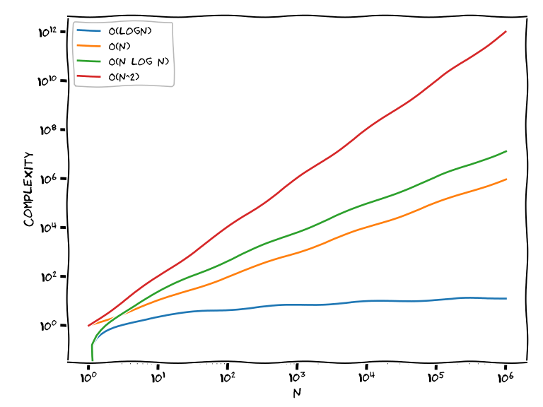
Just so that you understand where we are heading with this, look at figure Figure 5.1 for a second. For an input size of a million (\(10^6\)), if you are able to beat down the complexity of a given task from \(O(n^2)\) to \(O(n \log n)\)—which for a large class of problems is possible, e.g., by just working in Fourier space—you are moving down on the far right of our plot from the red to the green curve, reducing the running time by a factor \(\sim 10^5\). This might mean, e.g., that something that used to take a full day to run is now only taking one second. Not bad, eh?
And now, for something completely different, you might enjoy reading Knuth (1984). If it doesn’t make you laugh, start over from the beginning of the chapter. Repeat until you laugh out loud.
The Python program for the search of a maximum in a list was fairly simple. If you are wondering how you would go about understanding the complexity of an arbitrary algorithm or actual piece of code you might be handed over, I hear you. It can be pretty hard to make it starting from the first principle.
One obvious thing that you can do is to simply use the brute force: implement the algorithm in your favorite language, run it on input data of different size, time the execution and make a scatter plot of the running time vs. input size—you should get something resembling Figure 5.1. (Use caution: results may vary from run to run, and you will need to do some averaging and keep track of the uncertainties but, that all said, the thing works as advertised.)
If you are really brave, you can do everything by pure analysis: go ahead, count the steps of your algorithm (or elementary operations in your program, whatever that means) for any given input, and evaluate the average, best and worst-case scenarios. In practice, though, that generally involves sophisticated mathematics—remember Equation 5.1.
Fascinating as mathematics is, however, you can often gauge useful information about the behavior of a piece of code by just looking at it. A simple loop over the input data, for instance, implies a complexity \(O(n)\). How about two loops in sequence, one after the other? Remember: we are throwing away any multiplicative constant, so that’s again \(O(n)\). And how about two nested loops? Well, that brings us right into the land of \(O(n^2)\) which, most likely, means you are not doing things properly. We shall get back to this in a moment, but you got the message.
“Searching” is one of the words that appears next to “algorithm” more often, and this fundamental problem provides a natural setting to illustrate many of the topics we have glanced through in this chapter.
Say we want to write a function to search a given value in a list and return its index. The function should return \(-1\) is the target value is not in the list. (For simplicity, we shall assume that the list is homogeneous and contains integers, but this is irrelevant for our argument.) One possible way to go about it is:
def sequential_search(values: list, target: int) -> int:
    for i, value in enumerate(values):
        if value == target:
            return i
    return -1

l = [1, 2, 4, 6, 12, 32, 99]
print(sequential_search(l, 4))
print(sequential_search(l, 3))
2
-1What is the complexity of this sequential search? Easily said: there is one loop over the input, so \(O(n)\). Note the function returns as soon as we find the target, so, generally speaking, the loop is not guaranteed to iterate over the entire list, but that is irrelevant for our purpose: even if we visit half of the list on average, this is still \(O(n)\).
At a closer look, though, there is one important bit of information that we overlooked for this particular application: the input list that we passed to the function is sorted in ascending order. How can we turn that to our advantage?
def binary_search(values: list, target: int) -> int:
    left = 0
    right = len(values) - 1
    while left <= right:
        midpoint = (left + right) // 2
        value = values[midpoint]
        if value == target:
            return midpoint
        elif value < target:
            left = midpoint + 1
        else:
            right = midpoint - 1
    return -1

l = [1, 2, 4, 6, 12, 32, 99]
print(binary_search(l, 4))
print(binary_search(l, 3))
2
-1How would you explain in words this kind of binary search? Well, we start from the entire list, find the midpoint, and see if our target is larger or smaller than the corresponding value in the list. In the first case we restrict the search to the rightmost half of the list, and in the second case we restrict it to the leftmost half. No matter what, we cut the number of elements we have to look at by a factor of \(2\) at each step, and we iterate until either we find the target, or we realize the latter was not there in the first place.
What is the maximum number of steps (ops: we switched from elementary operation to steps again, but by now you know they are essentially the same thing from the standpoint of the complexity) that the algorithm needs to get to the finish line? By definition we are done when the width of the search window is one, which means \[ \frac{n}{2^{N_\mathrm{max}}} \approx 1 \quad \text{or} \quad N_\mathrm{max} \approx \log_2 n \] In the best case scenario we get the target at the first step. The average case, surprise surprise, is still \(O(\log n)\). Which, again, is a big thing: go look at Figure 5.1 and compare \(O(n)\) and \(O(\log n)\) for large \(n\)…
Before we move on, here is a slightly unrelated piece of advice. Binary search is a fairly standard algorithm and it is very unlikely that you will ever find yourself in need of implementing your very own custom copy. The Python standard library provides the bisect module
import bisect

def binary_search(values: list, target: int) -> int:
    # Check that the target value is not larger than all the elements,
    # as in that case bisect() would return an index outside the list.
    if target > values[-1]:
        return -1
    i = bisect.bisect_left(values, target)
    if values[i] == target:
        return i
    return -1

l = [1, 2, 4, 6, 12, 32, 99]
print(binary_search(l, 0))
print(binary_search(l, 1))
print(binary_search(l, 3))
print(binary_search(l, 4))
print(binary_search(l, 99))
print(binary_search(l, 100))
-1
0
-1
2
6
-1and numpy provides the searchsorted() function that is doing pretty much the same thing
import numpy as np

def binary_search(values: list, target: int) -> int:
    # Check that the target value is not larger than all the elements,
    # as in that case bisect() would return an index outside the list.
    if target > values[-1]:
        return -1
    i = np.searchsorted(values, target)
    if values[i] == target:
        return i
    return -1

l = [1, 2, 4, 6, 12, 32, 99]
print(binary_search(l, 0))
print(binary_search(l, 1))
print(binary_search(l, 3))
print(binary_search(l, 4))
print(binary_search(l, 99))
print(binary_search(l, 100))
-1
0
-1
2
6
-1That is, assuming that you remember that binary search exists when you need it, you are covered!
And “sorting” is the other big thing, when it comes to algorithms. Challenge of the day: write a small Python function that sorts an existing list. (Not that it really matters, but again assume that the list only contains integers.)
When prompted with such a problem, the first thing that comes to mind might be something along the lines: well, I can create an empty list, loop over the original list and, for each element, find its place in the new (sorted) list, with a second loop. That is:
def sloppy_sort(values: list) -> list:
    sorted_list = []
    for value in values:
        for i, item in enumerate(sorted_list):
            if value <= item:
                sorted_list.insert(i, value)
                break
        else:
            # Executed if the loop finishes without `break`
            sorted_list.append(value)
    return sorted_list

l = [10, 1, 8, 5, 2, 7, 3, 9, 4, 6]
print(sloppy_sort(l))
[1, 2, 3, 4, 5, 6, 7, 8, 9, 10]This work as advertised. Unfortunately, this is also horrible in at least two different, unrelated ways. For one thing the complexity of this algorithm is quadratic (i.e., \(O(n^2)\)); you can tell that right away from the two nested loops. In addition, you need to allocate a list that will grow to occupy the same memory as the original one.
else clauses on loops are a somewhat unusual Python feature that is described here.
The first thing is easy to fix: we have neglected the fact that, at any point in the execution of the program, the new list is sorted, and for the purpose to find the index at which we would insert the next item in the original list, we should do a binary search, which is \(O(\log n)\) instead of \(O(n)\).
import bisect

def slightly_better_sort(values: list) -> list:
    sorted_list = []
    for value in values:
        i = bisect.bisect_left(sorted_list, value)
        sorted_list.insert(i, value)
    return sorted_list

l = [10, 1, 8, 5, 2, 7, 3, 9, 4, 6]
print(slightly_better_sort(l))
[1, 2, 3, 4, 5, 6, 7, 8, 9, 10]You might be tempted to argue this is now \(O(n\log n)\) in complexity, while, unfortunately, the cost of a list insertion is linear, and we are still where we started from: \(O(n^2)\) and with a potentially big memory footprint. And this is where we stop guessing.
If you look at the wikipedia page for “Sorting algorithm”, you will find a long table of sorting algorithms available on the market. Although you are not an expert in algorithmic complexity by any reasonable metric, yet, you should be able to grasp the main take-away points from that table. In particular, the vast majority of the algorithms achieve the goal with a complexity of \(O(n\log n)\).
Curiosities aside (if you have spent enough time on the wikipedia page you have probably stumbled across the neat concept of Bogosort) the main message is again: refrain from re-inventing the wheel. Python lists come with a sort()
l = [10, 1, 8, 5, 2, 7, 3, 9, 4, 6]
l.sort()
print(l)
[1, 2, 3, 4, 5, 6, 7, 8, 9, 10]that will happily sort in place with reasonable performance. Full disclaimer: this uses Timsort under the hood, in case you care.
And now, for something completely different, if you happen to be into sorting algorithms and Hungarian folk dance, you might enjoy this article, along with the associated videos.
Data structures are often associated to algorithms in pedagogic resources, for the very good reason that in real life you often operate on complex structures, and at every step you need to know the cost of those operation in order not to be fooled. Take another look at the small snippet
def slightly_better_sort(values: list) -> list:
    sorted_list = []
    for value in values:
        i = bisect.bisect_left(sorted_list, value)
        sorted_list.insert(i, value)
    return sorted_list
Is this quadratic or not? Well, if it was only for the top-level loop and the binary search its complexity would be \(O(n \log n)\), but, as we said, list insertion is an expensive (as in \(O(n)\)) operation in Python, and since \(n\) beats \(\log n\) for large \(n\), the answer is: yes, this thing is quadratic.
The next obvious question is: how do I know what is the complexity of a given operation on a given type? Well, that is a very broad question, and the answer depends a lot on the specifics of the context we are working in. If all we are talking about is Python native types, the Time & Space Complexity Reference is a good resource.
(On a related note, and sadly enough, the page is also yet another evidence of how the AI hype is destroying communities all over the web: This wiki is in the process of being archived due to lack of usage and the resources necessary to serve it — predominately to bots, crawlers, and LLM companies. But so goes life.)
Understanding the precise behavior of a given type requires a detailed knowledge of how the object is implemented internally, and we just don’t have time for that—surely not for all the Python basic types. We shall take Python lists as an example, and see where this brings us.
In CPython, a list is basically a dynamic array of references to objects. Let’s try and parse it. At the very fundamental level, what we are storing in the underlying array are references to the objects—think about addresses in memory where the actual objects are (independently) stored. (That is to say: if you ask Python what is the memory footprint for the list, it will only take into account the memory occupied by the references, not that necessary for the actual items.)
One of the key design elements is that, while lists can be heterogeneous, with each item in the list having its own different size, addresses in memory are all integers of the same size. In addition to this contiguous array of integers, CPython lists contain two additional fields, expressing the current size of the list and the capacity of the underlying array of references. The clever part is: the reserved capacity is generally larger than the size, so that appending a new element to the list is fast, up to the point where you saturate the capacity, and you have to resize the whole thing.
The following, admittedly cryptic, snippet might or might not help grasping how a Python list is implemented internally. Use it if it makes it any sense to you, or just skip over otherwise.
import ctypes

class PyListObject(ctypes.Structure):
    _fields_ = [
        ("ob_refcnt", ctypes.c_ssize_t),
        ("ob_type", ctypes.c_void_p),
        ("ob_size", ctypes.c_ssize_t),
        ("ob_item", ctypes.POINTER(ctypes.c_void_p)),
        ("allocated", ctypes.c_ssize_t),
    ]

values = [42, "hello", 3.5]

internal = PyListObject.from_address(id(values))

print(f"List address in memory: {hex(id(values))}")
print(f"Reference counter: {internal.ob_refcnt}")
print(f"List length: {internal.ob_size}")
print(f"List capacity: {internal.allocated}")

for index in range(internal.ob_size):
    address = internal.ob_item[index]
    value = ctypes.cast(address, ctypes.py_object).value
    print(f"[{index}] address={address:#x}, value={value!r}")
List address in memory: 0x7fc38c6a9980
Reference counter: 1
List length: 3
List capacity: 4
[0] address=0x7fc3bfd38110, value=42
[1] address=0x7fc3ac49bae0, value='hello'
[2] address=0x7fc3ac0a1eb0, value=3.5We are now ready to go through all the basic operations that Python lists support and see if we can make sense of their average and worst-case complexity:
This was fairly quick, but again the Time & Space Complexity Reference is the place to start.
We promised we would not go through all the Python native types and we shall hold on to that promise, but since they are ubiquitous in the language, we shall make an exception for dictionaries.
A dictionary is an associative container, uniquely mapping a set of keys to a corresponding set of values, that CPython implements in the form of a hash table—a peculiar data structure interesting on its own. The basic idea is as follow:
The best part of hash tables is: getting, setting, inserting and deleting items all are \(O(1)\) in the average case, as all them basically imply a single evaluation of the hash function.
Of course this is an oversimplification. The devil in the details, and there’s a lot of details to be taken care of, here—devising the best hash function, handling collisions and optimizing the growing/shrinking strategy, just to name a few. The usual piece of advice applies here too: in the vast majority of cases you don’t want to implement a custom hash table from scratch. But bear with me and let’s continue this succinct overview.
First thing first, the hash function is supposed to be able to take literally anything as an input—a string, a number, you name it—and produce an integer withing a specified range in output. Generally speaking, there’s a number of desirable properties that we would like a good hash function to have:
(The last two are meant to minimize collisions, i.e., different keys going in the same hash. It goes without saying: no matter how careful you are, if the index space is finite there will always be collisions to handle.)
How does hashing work in Python? Well, for one thing Python provides the hash() builtin, that you can use to experiment.
for item in (-2, -1, 1, 1., 1.000000000001, "Hello"):
    print(f"{item} -> {hash(item)}")
-2 -> -2
-1 -> -2
1 -> 1
1.0 -> 1
1.000000000001 -> 2306049
Hello -> 7138970937675474918This is not nearly enough to reverse engineering the entire hashing infrastructure for native Python types, but it does provide some interesting clue as to what the basic design decisions for CPython were: integers, e.g., are hashed to themselves (expect for \(-1\), which is reserved as the C-level error return value), and numeric values that compare equal have the same hash value, even if they are of different types, as is the case for \(1\) and \(1.0\).
Can I hash literally any object in Python? Not quite—the following snippet, e.g., will raise an exception
l = [1, 2, 3]
print(hash(l))
--------------------------------------------------------------------------- TypeError Traceback (most recent call last) Cell In[14], line 2 1 l = [1, 2, 3] ----> 2 print(hash(l)) TypeError: unhashable type: 'list'
Why is that? Well, as it turns out, you can only hash immutable types, which, if you think about for a second, makes a lot of sense: the content of a mutable type could change after insertion into a dictionary, invalidating the stored hash-table position! (And yes: you can only use immutable objects as keys of a Python dictionary.)
Now it is really time to move on, but before we do take a look at this last snippet and make sure you understand what is happening:
d = {}
d[3] = "Hi there!"
print(d)

d[3.] = "How are you?"
print(d)
{3: 'Hi there!'}
{3: 'How are you?'}This is an odd corner of Python dictionaries—pay attention!