“Anyone who considers arithmetical methods of producing random digits is, of course, in a state of sin.” (John von Neumann, 1949)
I know, this is abused—you will find this very sentence quoted in any sensible resource about random numbers you might come across. But, on a second thought, it really encapsulates well the subject we are covering in this section: generating random sequences by means of arithmetical methods. Quite an oxymoron, eh?
2.1 Prelude: the wheel of fortune
If you were to ask an ordinary person on the street how they would go about drawing a random sequence, chances are that some sort of variant of the wheel of fortune would come up pretty high in the list of the most popular answers—provided that the person would care answering, of course. (I am sure you are familiar with at least one of the many popular TV shows that are based on the very concept of a wheel of fortune, but the Wikipedia entry on the subject is worth at least a quick read, because the idea seems very deeply rooted, and amusingly so, in western philosophy.)
Now, let us stop for a second and ask ourselves a very fundamental question: what is the magic in the wheel of fortune that makes its output so unpredictable? And I am going to stop for a second and let you think about it.
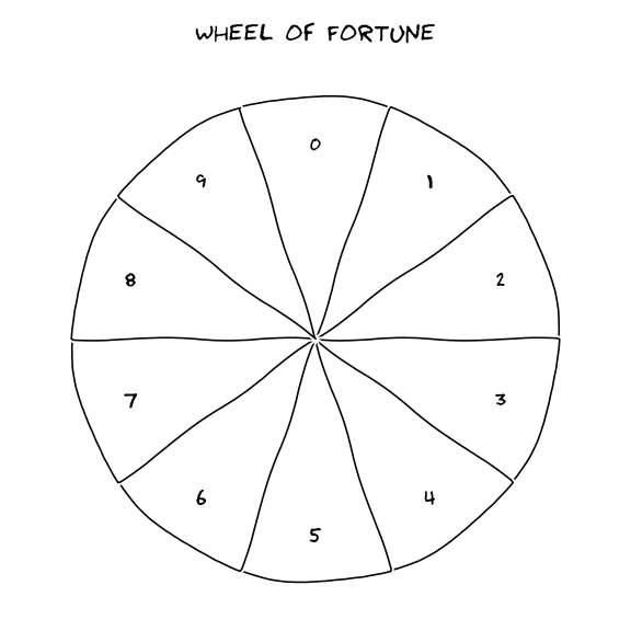
Figure 2.1: A wheel with 10 sectors.
You got it! It is the fact that the wheel wraps around at every turn. Let’s try and make this more quantitative with a toy model. For one thing we shall assume that the wheel has 10 segments, labeled with the integers from 0 to 9, that is, we are generating one decimal digit. If we say that \(\omega_0\) is the initial angular velocity that we spin the thing with, and \(\alpha\) the (modulo of) the angular deceleration, which for simplicity we shall assume constant in time, it is easy to show that the wheel stops when the angle \(\theta\) has changed by \[
\theta_0 = \frac{\omega_0^2}{2\alpha}.
\] If you have an uncertainty \(\sigma_\omega\) on \(\omega_0\) (which you always do), you will have an uncertainty of the final angular coordinate of \[
\frac{\sigma_\theta}{\theta_0} = 2 \frac{\sigma_\omega}{\omega_0}
\quad\text{or}\quad
\sigma_\theta = \frac{2\theta_0}{\omega_0} \sigma_\omega =
\frac{\omega_0}{\alpha} \sigma_\omega
\] That is: if you have a 1% uncertainty on \(\omega_0\), you end up with a 2% uncertainty on the final value of \(\theta\). And this is where things get interesting. If \(\theta\) was measuring a distance in a given direction and we were talking about a bocce-ball court (or a curling court, for what it’s worth) our model would describe a very poor device for generating random sequences: a good player can train to throw a ball (or a rock) very consistently (i.e., with a small error on the initial velocity) which means we can reliably predict where the ball itself will end up. Isn’t that the whole point of bocce, by the way?
But if we now go back to our wheel, where \(\theta\) wraps up at each turn, and we assume that \(\omega_0\) is large enough that the things does many turns, the situation is completely different. You might have noticed that the absolute error on \(\theta_0\) is proportional to \(\omega_0\) and, for any value of \(\alpha\) and \(\sigma_\omega\) there will be a value of \(\omega_0\) that is large enough for the error on \(\theta\) to be \[
\sigma_\theta \geq 2\pi.
\] When that happens, we have lost any capability to predict where the wheel will land. We might be able to predict roughly how many turns the wheel will do, but not the actual outcome. (In practice, for this to work, you might have to fine-tune \(\alpha\) based on some reasonable assumptions for \(\omega_0\) and \(\sigma_\omega\), but this is a technical detail.)
import numpy as npdef spin_wheel(omega0, alpha =0.1, num_segments =10):"""Spin our toy wheel of fortune! """# Calculate the overall angular advance until the wheel stops... theta = omega0**2./2./ alpha# ... wrap around at every turn, i.e., take the modulo 2 pi... theta = theta % (2.* np.pi)# ... and, finally, calculate the outcome by dividing by the angular with# of a sector and taking the integer part.returnint(theta / (2.* np.pi / num_segments))# Spin the wheel three times, changing the initial angular velocity by a small# amount (about 1%), and see that the output is basically random :-)print(spin_wheel(10.1))print(spin_wheel(10.2))print(spin_wheel(10.3))
1
7
4
If you got this far, you might be wondering: yeah, this is fun, but how about all this hype on the wheel of fortune? Weren’t we supposed to talk about random numbers? Well, as it turns out the fortune wheel is a surprisingly good mechanical analogy to how a typical pseudo-random (ops: did I just say “pseudo”?) number generator works. The mathematical equivalent of the concept of “wrapping around at every turn” is the modulo operation in ordinary integer arithmetic and it is interesting to note that, as we shall see in a moment, the modulo is a fundamental ingredient in all the generators that are relevant for everyday use. We shall briefly come back to modular arithmetic in section Section 2.4 but, before we do that, there’s a few thing we should sort out. In the meantime, L’Ecuyer (2017) provides an engaging and accessible account of the fascinating history of random number generators.
2.2 Random (and pseudo-random) sequences
While random numbers is an expression that you often find in the literature, you might have noticed that we prefer using random sequence. The reason is quite simple: there is no such a thing as a random number. “Here is a 5—is that random?” Clearly such a question makes little or no sense. What makes sense, instead, is the concept of a random sequence. That one we like.
So let’s say we have a sequence \(X_n\) of integers with \(0 \leq X_n < m\). (In our toy wheel-of-fortune setup, e.g., we had \(m = 10\), but we anticipate that, for all practical purposes, we shall be interested in much larger values for \(m\).) To be concrete, let’s say that we spin our wheel of fortune and get \[
X_n = 2, 5, 1, 3, 9, \ldots
\] Can we confidently say that this is a random sequence? As it turns out, this is a very hard question that has no good answer. We shall briefly come back to the issue in Section 2.8, but we anticipate that, while there are obvious properties that we would like from a truly random sequence (such as the fact that all the possible elements appear with the same frequency, within the expected statistical fluctuations), there is no easy direct proof that a given sequence is random. Usually people apply an entire battery of standard tests and declare that a given generator is random if the sequences it produces pass all the tests.
It is also worth mentioning that, while the sequence \[
X_n = 0, 1, 2, 3, 4, 5, \ldots
\] definitely does not appear to be random (although all the digits are equi-distributed) in a truly random setting it is just as likely to appear as any other—including the first one we have shown. You get it: assessing randomness is difficult.
Let us turn for a second to a slightly different question: how could I conceivably generate a random sequence? Well, arguably I could use a truly random natural process. Although, when you think really hard about this, it is far from trivial to devise a truly random process, True Random Number Generators (TRNGs) do exist, and serve very precise purposes. Have a look at www.random.org for a good example, and a good source of information on the topic. What we are mainly concerned here, though, is how to programmatically generate deterministic sequences by means of arithmetical methods that behave as if they were random. Such generators are called Pseudo-Random Number Generators (PRNGs) and are the main topic of this chapter.
The distinction between TRNG and PRNG is a fundamental one, and its importance can hardly be overstated. The former are by definition aperiodic and non deterministic (i.e., you cannot repeat the same sequence twice) and tend not to be very efficient. Yet, if you want to run a lottery, you should probably have a look at this article about the the Michael Larsen incident (amusing reading, I promise) before you consider opting away from a TRNG.
PRNGs, on the other hand, are typically very efficient and have the advantage that you can regenerate a given sequence as many times as you want. This is definitely your first choice for a Physics simulation—really, it is a no-brainer.
2.3 Tables
There has been a time when tables (and even huge ones) of (true) random digits were actually a thing. The most famous instance of such endeavors is probably the book A Million Random Digits with 100,000 Normal Deviates published in 1955 (and re-issued in 2001) by the RAND corporation. If you have 70 euros to spare you can buy one of the last paper copies available online. (The reviews of the book are quite funny, too.)
Nuisance to use. Memory was precious in the old days. Both motivated the development of alternative means for producing random numbers.
2.4 Digression: modular arithmetic
2.5 Pseudo-random sequences via recurrence
If you happen to be under impression that pseudo-random number generation is a solved problem, you couldn’t be more wrong. For many years linear congruential generators (LCG) have been the de-facto standard. In 1997 Matsumoto and Nishimura (1998) caught the entire World by surprise when they published the Mersenne Twister (MT) algorithm: with a stunning period of \(2^{19937} −1\) and many other desirable properties it immediately underwent widespread adoption, and still is the default engine in many programming languages (including Python) and statistical packages. It took several years for some definite shortcomings and limitations now widely recognized to emerge. In 2014 O’Neill (2014) published the idea of a family of permuted congruential generators (PCG), and this is a notable case of an idea that has never been published in a formal scientific paper, has been harshly criticized in a number of blogs and other informal forums on the web (see, e.g. here), and yet had real-world impact, as PCG is the default random generator in numpy (and the related discussion is a good testament as to how difficult is agreeing on what the best PRNG is).
The simplest way to generate a pseudo-random sequence is a by a recurrence relation of the type \[
X_{n+1} = f(X_n) \bmod m
\tag{2.1}\] where \(X_{n+1}\) and \(X_n\) are non-negative integers, \(m\) is called modulo, and \(f(x):~\mathbb{N} \rightarrow \mathbb{N}\) is a suitable function. (More on this later.) The idea is that you start from a seed\(0 \leq X_0 < m\) and let all the other numbers flow from Equation 2.1.
Although more complex schemes can (and have been) devised, this very basic setting is a good one to discuss some of the general properties that are common to all pseudo-random sequences. The most obvious one is perhaps the fact that all the numbers in the sequence satisfy \(0 \leq X_n < m\), which is to say that at most \(m\) distinct values can be produced. It follows that, sooner or later, we are bound to stumble across a number that we have already visited, and from that point on we just go on in circle. We can phrase this very thing in a slightly different way by saying that, ultimately, any pseudo-random sequence is periodic. In our particular case the period \(p\) satisfies \(p \leq m\). This is not necessarily an issue if \(p\) is large enough, but definitely important to keep in mind.
At the very basic level, some of the good properties that a PRNG should have include
a long period;
high speed (i.e., \(f(x)\) should be easy to calculate on a computer);
a small memory footprint;
good statistical properties (for one thing we will want that any reasonably long subsequence is equi-distributed in the \([0,~m]\) interval, but as we shall see in a moment there are many other desirable properties).
We emphasize that, while having a long period is important, it is not by any means the only important thing. The sequence \[
X_{n+1} = X_n + 1 \bmod m \quad \text{e.g.} \quad 0,~1,~2\ldots m
\] provides the maximum period \(m\), but it is obviously not random.
Before we move on, you feel be uncomfortable with the fact that we are dealing with integers. Most of our simulations live in the realm of floating-point numbers, and when do we get to that? Well, you just do \[
u_n = X_n / m
\] and here is you sequence of integers turned into a sequence of floating-point numbers between \(0\) and \(1\). (It goes without saying, these are by all means plain, rational numbers, but this is as far as floating-point arithmetics goes on a digital computer, and we already knew that.) Appendix ??? provides a cursory summary of floating point arithmetics; in the next chapter we shall discuss how we turn an equi-distributed sequence in the \([0,~1]\) interval into more interesting things.
2.6 Middle square
Devised by John Von Neumann at the turn of the 1940s, the middle-square (MS) method if often regarded as the oldest practical method to produce pseudo-random sequences, as well as an archetypal examples of all the idiosyncrasies that a good generator should stay away from. This blog post is a beautiful reading on the matter.
The underlying algorithm that the name middle square is meant to convey is the following: given a seed \(X_0\) with \(n\) digits, take its square \(X_0^2\) (this will have at most \(2n\) digits, and you can actually make it a \(2n\)-digits number by padding with zeros on the left side) and select the \(n\) digits in the middle of its numeral representation; this is the next number in the sequence. That is, assuming that we are working with four decimal digits, if we start with 3333, we square it to get 11108889 and the next number in the sequence is 1088; then comes 1837. And so on and so forth.
Quick digression. If you paid attention you will notice that what we are doing is mixing numbers and numerals: calculating the square has a meaning that is independent from the base we are using, but taking the \(n\) mid digits is something that operates on the string representation of the number, not the number itself. That is, using decimal or binary digits are two different things in this context. Going back to our previous example, decimal 3333 translates to 0b110100000101 (12 binary digits), 11108889 to 0b101010011000001000011001 (24 binary digits), and if we get rid of six digits on both sides we get 0b011000001000, i.e., decimal 1544. The two things do not roundtrip. Not a big deal, but definitely something to be aware of. You will also notice that for the very concept of selecting the \(n\) digits in the middle not to be ill-defined, \(n\) must be even to start with.
Back on track. How do I translate selecting the \(n\) digits in the middle in a way that can be expressed in a programming language? Well, you could convert the number into a string and operate on that, but at a second glance it is easy to see that you can actually do it with a combination of the modulo operator and the integer division. In Python the thing might read vaguely like:
def next_middle_square(x):"""Calculate the next element in a middle square sequence (4 decimal digits). """return (x **2//100) %10000value =3333# The number following 3333 should be 1088.value = next_middle_square(value)print(value)# The number following 1088 should be 1837.value = next_middle_square(value)print(value)
1088
1837
All right. What can we say on the properties of the sequence? Well, for one thing, it fits in our definition given by Equation 2.1 as we can wite the recurrence relation as \[
X_{n + 1} = \left\lfloor \frac{X_n}{b^\frac{e}{2}} \right\rfloor \bmod b^e
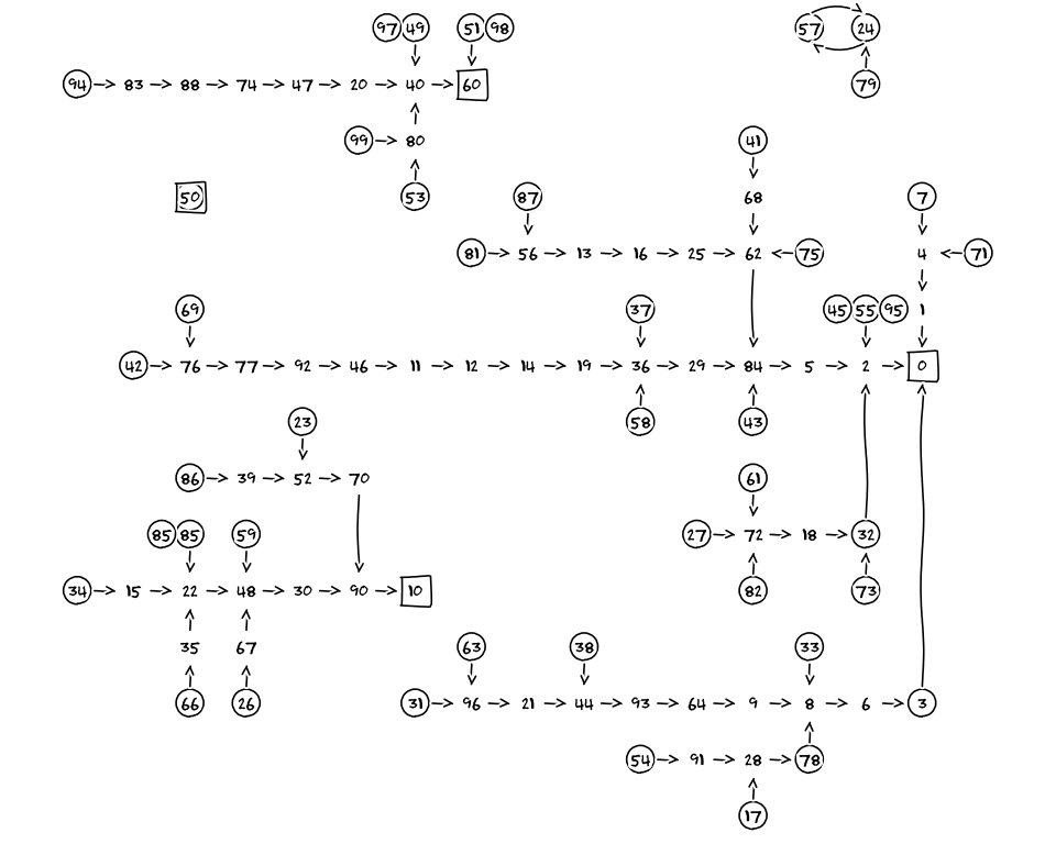
\] where the brackets indicate the integer division ignoring the reminder, \(b\) is the base (e.g., 10, or 2) in which we operate, and \(e\) is the number of digits we are targeting. What can we say about the period we are expecting? Does it depend on the seed? And how about the other statistical properties? This is where things get a little bit difficult, as this is a hard problem to attack mathematically. (And, admittedly, not a very interesting one from any practical standpoint.) But since we have computers, it is very easy to attack it with brute force, and Figure 2.2 shows all the possible sequences that we might ever get with two decimal digits.
Figure 2.2: Full directed graph of all the possible sequence for a 2-decimal digits middle-square generator.
A few directions to read the graph. The numbers surrounded by a circle (e.g., 94) are all of those that you only visit if you use them as a seed to start with—they have no other input leading into them. There are exactly four numbers (with two decimal digits) that are transformed into themselves by the middle-square algorithm, and they are: 0, 10, 50 and 60 (make sure you can verify that with pencil and paper); for obvious reasons, they are called fixed points, and they are surrounded with a square in the graph. As soon as one stumbles across a fixed point, the sequence is stuck into an infinite cycle of length one. Not good. 50 is doubly peculiar, in that is both a fixed point, and one that has no input. You only visit it if you use it as a seed, and if you do that you never see anything different; a nice example of a cute little sequence of length 1. 57 and 24 are also peculiar in that they are transformed into each other, and make it for the only non-trivial cycle (of length 2, in this case) that one encounters with two decimal digits. Although the theoretical maximum period in this case is 100, the two longest sequences across all possible seeds are the ones going from either 42 or 69 to 0, and they both have exactly 15 elements. All other sequences are shorter than that, and most of them much shorter. Disappointing.
Does this mean that all is lost, or is it rather than two digits are too few, and the thing is well behaved with longer number? How about middle-square sequences with 12 decimal digits? Are those any good? I am afraid the answer is no, unfortunately. No matter how many digits you use, the middle square method tends to be trapped in fixed points or relatively short cycles. The median sequence length scales as the square root of the modulo. With 12 digits you have a theoretical maximum period of \(10^{12}\) and yet the typical sequence has a period that is a million times shorter. Not exactly an example of efficiency.
2.7 Linear congruential generators
Linear congruential generators (LCG) are among the most studied and well understood PRNG available, and have been widely used since the early 1950s. First discussed in a paper by D. H. Lehmer, they take the general form \[
X_{n+1} = (a X_n + c) \bmod m
\tag{2.2}\] where \(a\) is called the multiplier, and \(c\) the increment.
A cursory look at the following LCG for two decimal digits clearly show that, unless we devise a good strategy for choosing the underlying constants, a linear congruental generator is not necessarily better than the middle-square—which we said it was terrible.
m =100a =40c =8seed =33sequence = []value = seedwhile value notin sequence: sequence.append(value) value = (a * value + c) % mprint(f"Sequence length: {len(sequence)}{sequence}")
Sequence length: 2 [33, 28]
(What is happening, here, is that the second value, 28, is transformed into itself, and we are stuck with a sequence of length 2. Disappointing.)
The good news is that we have a good amount of well understood theory that goes with this class of generators. More specifically, the Hull–Dobell theorem states that all we have to require to guaranteed the maximum period \(m\) is that
\(m\) and \(c\) are coprime (i.e., their greatest common divisor is 1);
\(a - 1\) is divisible by all prime factors of \(m\);
\(a - 1\) is divisible by 4 if \(m\) is divisible by 4.
Full disclaimer: you will not be qualified to design new PRNGs after just reading this document anyway, and it is perfectly ok if you have no idea of how you would go about demonstrating this. It is even ok if you do not commit to permanent memory the precise conditions of this theorem. But let’s take a closer look at what they imply in this particular case. The prime factors of \(m\) are 2 and 5, so we want \(a - 1\) to be divisible by both. Actually, since \(m\) is divisible by 4, we want \(a -1\) to be divisible by both 4 and 5, which is to say \[
a \bmod 20 = 1
\] This leaves us with the relatively small set \(a \in \left\{ 1, 21, 41, 61, 81\right\}\). And it should not be difficult to convince yourself that 1 would be a terrible choice. (Not convinced? Pick \(a = 1\) and \(c = 1\), and you have created a beautiful counter—sure enough it reaches the longest possible period \(m\), but it does not look very random, does it?) The other thing is that we want \(c\) coprime with 100, which means that it should be odd and not a multiple of 5—how about 11? All right, we might have a winner!
m =100a =21c =11seed =33sequence = []value = seedwhile value notin sequence: sequence.append(value) value = (a * value + c) % mprint(f"Sequence length: {len(sequence)}{sequence}")
Whoho! This sequence is indeed starting from 33 and is happily cycling through all the possible numbers between 0 and 99 included, with no obvious patterns, before it goes back to where we started. Note that the fact that the trick works with 33 as a seed implies that it also works with any other seed. And we can now do the same wit, say, 12 decimal digits and get actual random numbers.
On a second thought: are we really happy with this? Look at the least significant digit of the elements in the sequence: 3, 4, 5, 6, 7… It doesn’t look random, does it? As it turns out, this is a well understood fact too: with such a small number of digits, there is essentially no way for the output not to show patterns. (There is also a more subtle reason, that is, we have chosen the multiplier to be a power of the base we are working with, but this is becoming too technical.) The point is: if you are careful, things do get better with larger number, but by all means having a long period is not the end of the story. Which brings us to the next question: now that we start dealing with candidate sequences that are not obviously flawed by just looking at them with the naked, eye, how do we tell if any particular one is really good?
2.8 Tests for randomness
When discussing the tests for randomness, the specifics depend on what we are testing, exactly, e.g., \(X_n\) as integers vs. \(u_n\) as floating-point numbers in the \([0,~1]\) interval.
If we concatenate all the subsequent \(X_n\) and treat our sequence as an un-interrupted stream of decimal digits, a few obvious desirable things immediately come to mind. For one thing we would like each digit to appear with the same probability \(1/10\) in the sequence. (We note that this is hardly enough for the thing to appear as random, as a simple counter \(X_n = 0,~1,~2,~3\ldots\) trivially satisfy this.) We may ask that pairs of subsequent identical digits, e.g. \(2,~2\), or \(7,~7\), appear with the expected probability \(1/100\), and this can be easily generalized to triplets, quadruplets or, really, arbitrary high multiplicity.
In reality, there is a nearly unlimited number of properties that one can list and, in absence of a single test that can qualify a given sequence as good enough in terms of randomness, the best that one can do is feed their generator to a full battery of tests, and hope that it passes them all.
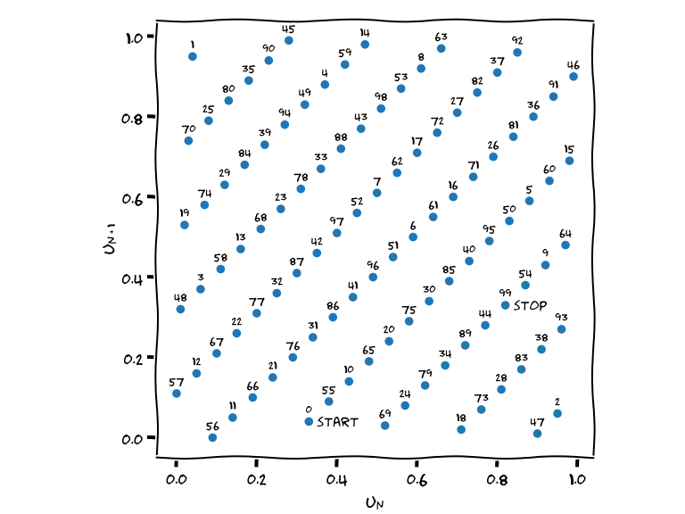
There in one, special test, though, that is worth at least a cursory discussion as it offers interesting insight into the very basic process of generating random numbers by arithmetical means. It is called the spectral test, and is based on a nice little paper by Marsaglia (1968) titled Random numbers fall mainly in the planes. Let’s go back for a second to the simple LCG we have discussed in the previous section—more specifically to the maximum-period sequence we have obtained in the last snippet by carefully choosing the multiplier and the increment. Figure 2.3 shows how pairs of successive point \(u_n~,u_{n+1}\) are distributed in the cartesian plane. (Make sure you grasp the meaning of the plot. This is in \(u_n\) space, i.e., we divided the \(X_n\) by the modulus, and the small text label indicate the index in the sequence at which each number occurs: the first point is \(0.33,~0.04\), after which we jump to the upper-left corner \(0.04,~0.95\), then to the opposite corner \(0.95,~0.06\) and so on and so forth.)
Figure 2.3: Representation of the \(u_n,~u_{n+1}\) ordered pairs for the simple linear congruential generator with maximum period discussed in the previous section. The decimal integers have been converted into floating-point numbers in the \([0,~1]\) interval dividing by the modulus. The small numbers indicate the order of appearance in the sequence.
Well, it is fair to say that this is looking anything but random. At a second though, maybe this is not really unexpected. We are pretending to generate random real numbers, but under the hood all we are doing is truncating stuff in the \([0~,1]\) interval to and accuracy of \(1/m\) and therefore we are bound to be unable to properly fill the plane in this representation. With a ridiculously small modulo such as 100 things look understandingly horrible, and one has hope that with a much larger \(m\) things are better—and indeed they are—but nonetheless this is a feature that cannot be overcome and we need to keep it in mind. Marsaglia (1968) makes this all quantitative for LCG, showing that the output of a LCG with modulo \(m\) lie on at most 14 straight lines. In Figure 2.3 we do see 10 lines oriented at \(45^\circ\), so our generator is pretty much as good as it gets with two decimal digits.
The thing can in fact be generalized from 2 to \(n\) dimensions (e.g., for \(n=3\) we are dealing with triplets \(u_n,~u_{n+1},~u_{n+2}\) in the volume, for \(n=4\) with quadruplets, and so on and so forth), and the basic content of Marsaglia’s theorem is that the output n-tuples from a LCG will lie on at most \[
(n! m)^{\frac{1}{n}}
\] hyperplanes. For \(n=2\) and \(m=2^{128}\), for instance, this gives about \(2 \times 10^{19}\) lines—something we hardly have to worry about. (And yet, if we are looking at \(n=10\) we are talking about only 32296 hyperplanes.)
2.8.1 The worst LCG ever
The spectral test brings us to another piece of random number folklore: RANDU, now universally dubbed as one of the most ill-conceived PRNGs to have ever seen widespread use. Originally introduced by IBM at the end of the 1950s, RANDU is defined as a (purely) linear congruental generator with modulo \(m = 2^{31}\), multiplier \(a = 65539\) and increment \(c = 0\)\[
X_{n + 1} = 65539 \; X_n \bmod 2^{31}
\] This was done purely on efficiency consideration, with no regard to the statistical quality of the output: since \(65539 = 2^{16} + 3\), the recurrence relation can be rewritten as \[
X_{n + 1} = ((X \ll 16) + X + (X \ll 1)) \bmod 2^{31}
\] which on a 32-bit binary computer only involves bit shifts, additions and a truncation (the final modulo), all of which could be done very efficiently in hardware.
Phrased in a slightly different way, RANDU was blazingly fast on a typical computer of the time. And yet it can be shown that it fails spectacularly the spectral test with \(n \ge 3\), as the output triplets only sample 15 planes in the unit cube against a theoretical maximum of 2344.
2.9 Modern generators
Cover very quickly F2-linear pseudorandom number generators, and particularly MT and Xoshiro. Also PCG makes it for an interesting story.
Include a few words about crypto generators, and mention the relevant Python module.
2.9.1 Period: is that really important?
While quoting wall-clock time when discussing computer operations is always a little bit silly, nowadays most modern generators run at a speed of a few ns per call on a typical laptop. It would take a time equal to the current age of the universe to generate \(10^{27}\) random numbers, if that was the only thing that we were doing. I’ll give you 1000 parallel streams and make that \(10^{30}\). For comparison, \(2^{128} \approx 3.4 \times 10^{38}\) (that is, almost a billion larger), \(2^{256} \approx 1.2 \times 10^{77}\) (which is only three orders of magnitude short of the number of protons in the universe), and \(2^{19937} \approx 10^{6000}\). (You will have to resort to your high-school knowledge of the logarithms to calculate it, because if you try in a Python prompt you will get an overflow error.)
Now, an obvious question arise: do we really need such a ridiculous period from a PRNG?
On the flip side of the story, \(35! \approx 10^{40}\), so be aware that, if you are into combinatorial problems, with a period as short as \(2^{128}\) you will not be able to generate all the possible random permutations of a set of 35 elements. Somebody (see, e.g., [this paper]) think that is actually a big deal.
2.10 What am I using under the hood?
It is fair to say that LCG are pretty much dead, nowadays. Many popular programming languages and data-analysis program, while offering many options, default to the MT19937 version of the Mersenne Twister algorithm, although its limitations are widely recognized. The ROOT documentation for the TRandom class reads verbatim “this is a very BAD Generator, not to be used” referring to MT19937, and yet that is used to instantiate the global pointer to the ROOT generator. So goes life. Meanwhile the PCG and Xoshiro families of PRNG are gaining traction. Here is a largely incomplete survey of the situation as of 2026.
Table of the default random generators in some widely used programming languages and statistical frameworks.
Exercise 2.1 (Middle square) Characterize the middle-square method for producing random numbers with \(n\) decimal and/or binary digits at least up to \(n = 8\), and possibly more. In each case identify all the fixed points and possible loops, and calculate the median period across all possible seeds. Verify that the latter scales as \(\sqrt{n}\).
Exercise 2.2 (RANDU) Devise a simple toy problem where the RANDU PRNG clearly fails beyond the expected numerical precision, and verify that a modern generator (e.g., MT or PCG) fixes the problem.
Blackman, David, and Sebastiano Vigna. 2021. “Scrambled Linear Pseudorandom Number Generators.”ACM Trans. Math. Softw. 47 (4). https://doi.org/10.1145/3460772.
L’Ecuyer, Pierre. 2017. “History of Uniform Random Number Generation.” In Proceedings of the 2017 Winter Simulation Conference. WSC ’17. Las Vegas, Nevada: IEEE Press.
Marsaglia, George. 1968. “Random Numbers Fall Mainly in the Planes.”Proceedings of the National Academy of Sciences of the United States of America 61 1: 25–28. https://api.semanticscholar.org/CorpusID:30098699.
Matsumoto, Makoto, and Takuji Nishimura. 1998. “Mersenne Twister: A 623-Dimensionally Equidistributed Uniform Pseudo-Random Number Generator.”ACM Trans. Model. Comput. Simul. 8 (1): 3–30. https://doi.org/10.1145/272991.272995.
O’Neill, Melissa E. 2014. “PCG: A Family of Simple Fast Space-Efficient Statistically Good Algorithms for Random Number Generation.” HMC-CS-2014-0905. Claremont, CA: Harvey Mudd College.