Let us assume that we want to calculate the definite integral \[
I = \int_0^1 \frac{1}{1 + x^2} dx.
\] Before you ask: there is nothing really special about this function, except the fact that it is smooth, and its primitive has a simple, analytical form—and therefore our integral is readily evaluated: \[
I = \arctan(1) = \frac{\pi}{4}.
\]
How can we put a generator of equi-distributed random numbers to use to estimate this integral?
3.1 The hit-or-miss method
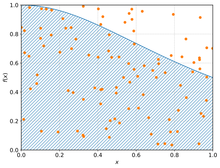
On of the features of the integration region we have chose for our example is that it can be enclosed in the unitary square—so why don’t we go ahead and throw a whole bunch of random points in this square and count how many of them fall below the curve? The fraction of the latter should asymptotically tend to \(I\).
import numpy as npfrom matplotlib import pyplot as pltrng = np.random.default_rng(313)n =100def f(x):return1./ (1.+ x**2.)# Evaluate the function on a grid.x = np.linspace(0., 1., 100)y = f(x)# Throw some random numbers in the unitary square.px = rng.random(size=n)py = rng.random(size=n)# Count how many of them fall below the curve.k = (py < f(px)).sum()I = k / nplt.plot(x, y)plt.gca().fill_between(x, 0, y, facecolor="none", edgecolor="tab:blue", hatch="///", linewidth=0)plt.plot(px, py, "o")plt.axis([0., 1., 0., 1.])plt.xlabel("$x$")plt.ylabel("$f(x)$")print(f"{k}/{n} = {I} (expected {np.pi /4.})")
79/100 = 0.79 (expected 0.7853981633974483)
This works as advertised, and generally goes under the name of hit-or-miss Monte Carlo integration. (Spoiler alert: it is unlikely that you will use it extensively, but the technique is germane to the one bearing the same name that is used for sampling distribution, so it is instructive to take a look.)
Let us look at this technique in some more details. Let \(D\) be our domain of integration (with area \(I\)) and \(R\) (typically a rectangle, with area \(A_R\)) the region we are throwing our random points in: assuming that we throw \(n\), uniformly distributed random points in \(R\), and \(k\) of them end up inside \(D\) the quantity \[
\hat{I} = \frac{k}{n} A_R
\tag{3.1}\] is an unbiased estimator for \(A_D\), in the sense that \[
E[k] = n \frac{I}{A_R}
\quad\text{and therefore}\quad
E[\hat{I}] = I.
\]
How do we estimate the uncertainly associated to our estimator? Well, \(k\) is a binomial random variable with \(p = \frac{I}{A_R}\) and therefore \[
\text{Var}(\hat{I}) = \frac{A_R^2}{n^2}\text{Var}(k) =
\frac{A_R^2}{n^2} np(1 - p) = \frac{I (A_R - I)}{n}
\quad\text{and}\quad
\sigma_{\hat{I}} = \sqrt{\frac{I (A_R - I)}{n}}
\]
Let’s look at this expression for a second. First thing first, we notice that this estimates includes the unknown integral \(I\)—this is sometimes called an a priori error analysis. This will suffice for our scope: we can always plug in our estimate of \(I\) and get an approximate expression that only depends on measured quantities: \[
\sigma_{\hat{I}} \approx \sqrt{\frac{\hat{I} (A_R - \hat{I})}{n}}.
\tag{3.2}\]
This allows to derive a number of interesting facts. The uncertainty on the integral asymptotically tends to zero for large \(n\) with a convergence rate of \[
\sigma_{\hat{I}} \propto n^{-\frac{1}{2}},
\] which, as we shall see, is a basic property of Monte Carlo integration, independently of the number of dimensions of our problem. The multiplicative constant for the convergence depends on the actual values of \(I\) and \(A_R\), and it is more conveniently expressed in relative terms: \[
\frac{\sigma_{\hat{I}}}{\hat{I}} \approx
\sqrt{\frac{(1 - \varepsilon)}{\varepsilon}} n^{-\frac{1}{2}}
\quad\text{where}\quad
\varepsilon = \frac{\hat{I}}{A_R}.
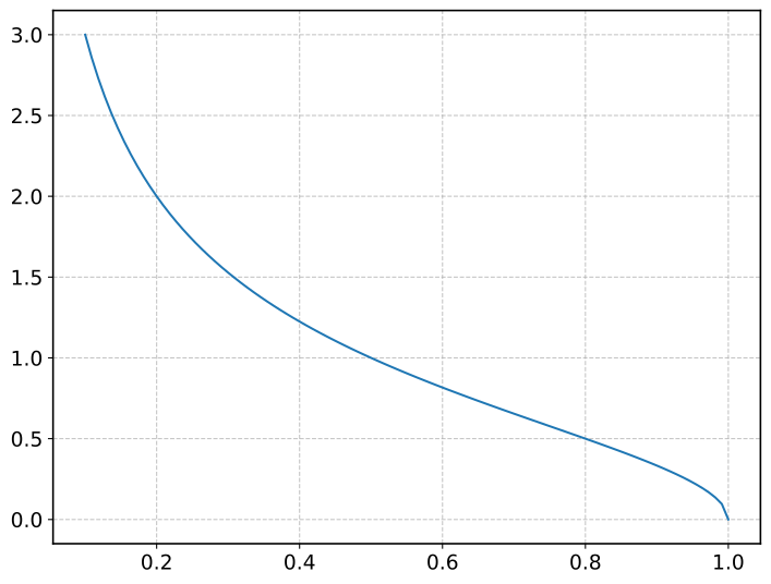
\] Interesting: the constant only depends on the ratio of the original integral to the area of the bounding region. How? Easily shown!
That is: for best performance you want the bonding region to be as close as possible to your integration domain—-when the two are the same the uncertainty is exactly zero, as you know \(A_R\) and, therefore, you know the answer. (Keep in mind this is not always easy to achieve, as it’s easy to throw random points uniformly distributed in a rectangle, not so much in an arbitrarily complex region.) For \(\varepsilon = 1/2\), which you can take as a typical example of an integration setup that is not ill-posed, the constant is equal to unity. Easy to remember.
And here is a fully fledged, vectorized Python function that will calculate the definite integral (and associated uncertainty) of a generic one dimensional function by means of a hit-or-miss Monte Carlo technique.
import numpy as nprng = np.random.default_rng(313)def hit_or_miss_integral(func, a, b, ymin, ymax, n):"""Calculate the definite integral of a function by means of the hit-or-miss Monte Carlo method. Note this requires ymin <= f(x) <= ymax on the [a, b] interval. Arguments --------- func : callable The integrand f(x). It must accept a NumPy array as the only argument and return an array of function values with the same shape. a : float Lower bound of the integration interval. b : float Upper bound of the integration interval (must be > a). ymin : float Lower vertical bound of the integration interval. ymax : float Upper vertical bound of the integration interval. n : int Number of points for the Monte Carlo sampling. Returns ------- I : float Estimate of the integral. sigma_I : float Estimated one-standard-deviation statistical uncertainty of the integral estimate. """ A_R = (b - a) * (ymax - ymin) x = rng.uniform(a, b, size=n) y = rng.uniform(ymin, ymax, size=n) I = np.mean(y < func(x)) sigma_I = np.sqrt(I * (A_R - I) / n)return I + (b - a) * ymin, sigma_Idef f(x):return1./ (1.+ x**2.)I, sigma_I = hit_or_miss_integral(f, 0., 1., 0., 1., 100000)target = np.pi /4.rel_error =abs(I - target) / targetprint(f"Integral = {I:.4f} +- {sigma_I:.4f} (relative error: {rel_error:.1e})")
Integral = 0.7870 +- 0.0013 (relative error: 2.0e-03)
3.2 The sample-mean method
We can recast the problem of calculating a definite integral \[
I = \int_a^b g(x) dx
\] in a completely different fashion. If we take \(x\) to be a continuos random variable uniformly distributed between \(a\) and \(b\), i.e., \[
p(x) = \frac{1}{(b - a)} \quad\text{for}\quad a \leq x \leq b
\] we might take advantage of the fact that the probability density function is a simple constant and rewrite our integral as an expectation value for \(g\): \[
I = (b - a) \int_a^b g(x) p(x) dx = (b - a) E[g(x)].
\] At a second look, this is hardly surprising: the integral of a function over an interval is equal to the width of the interval, times the mean value of the function—who would have guessed?
This, in turn, is opening up an entirely new avenue for us, as we can approximate the true average with the sample average over a finite number of random variates \(x_i\) equi-distributed between \(0\) and \(1\) (i.e., exactly the thing that we just became good at simulating) \[
\hat{I} \approx \frac{(b - a)}{n}\sum_{i=1}^n g(x_i).
\tag{3.3}\] It is easy to see that this, too, is an unbiased estimator of the original integral, in the same way the sample mean is an unbiased estimator of the mean of a distribution.
(Note we are not sampling the original function \(g(x)\)—we are applying\(g(x)\) to a sample or random deviates equi-distributed between \(0\) and \(1\).)
How do we estimate the uncertainty, this time around? Well, once again we have to calculate the variance of our estimator \[
\text{Var}(\hat{I}) =
\frac{(b - a)^2}{n^2} \text{Var} \left( \sum_{i=1}^n g(x_i) \right) =
\frac{(b - a)^2}{n^2} \sum_{i=1}^n \text{Var}(g(x_i)) =
\frac{(b - a)^2}{n} \text{Var}(g(x))
\]
Now, written in this form this is not particular nice looking, as the variance of our function contains both the original integral and the integral of \(g^2(x)\), which is most likely even more difficult—you will see the expression made explicit as \[
\text{Var}(\hat{I}) =
\frac{1}{n} \left[ (b - a) \int_a^b g^2(x) dx - I^2 \right] =
\frac{(b - a)}{n} \int_a^b \left( g(x) - \frac{I}{(b - a)} \right)^2 dx.
\]
Sampling comes to rescue, again, as we can approximate the variance of the function as \[
\text{Var}(g(x)) \approx
s^2 = \frac{1}{n - 1} \sum_{i=1}^n (g(x_i) - m)^2
\quad\text{where}\quad
m = \frac{1}{n} \sum_{i=1}^n g(x_i) = \frac{\hat{I}}{(b - a)}.
\] That is: \[
\sigma_I \approx (b - a) s n^{-\frac{1}{2}}
\quad\text{or}\quad
\frac{\sigma_I}{\hat{I}} \approx \frac{s}{m} n^{-\frac{1}{2}}
\tag{3.4}\]
Here is a complete Python implementation.
import numpy as nprng = np.random.default_rng(313)def sample_mean_integral(func, a, b, n):"""Calculate the definite integral of a function by means of the sample mean Monte Carlo method. Arguments --------- func : callable The integrand f(x). It must accept a NumPy array as the only argument and return an array of function values with the same shape. a : float Lower bound of the integration interval. b : float Upper bound of the integration interval (must be > a). n : int Number of points for the Monte Carlo sampling. Returns ------- I : float Estimate of the integral. sigma_I : float Estimated one-standard-deviation statistical uncertainty of the integral estimate. """ x = rng.uniform(a, b, size=n) I = np.mean(func(x)) sigma_I = (b - a) * np.std(func(x)) / np.sqrt(n)return I, sigma_Idef f(x):return1./ (1.+ x**2.)I, sigma_I = sample_mean_integral(f, 0., 1., 100000)target = np.pi /4.rel_error =abs(I - target) / targetprint(f"Integral = {I:.4f} +- {sigma_I:.4f} (relative error: {rel_error:.1e})")
Integral = 0.7851 +- 0.0005 (relative error: 3.7e-04)
3.3 Convergence
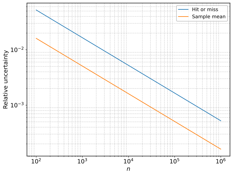
You might have noticed that, in our particular case, the standard error for the sample mean is smaller that that for the hit-or-miss integration, and so is the relative deviation of the central value from the known target.
The example function we have picked to illustrate the problem is easy enough that the standard error can be analytically calculated for both techniques \[
\frac{\sigma_I^\text{HM}}{\hat{I}} = \sqrt{\frac{4}{\pi} - 1} \; n^{-\frac{1}{2}}
\quad\text{and}\quad
\frac{\sigma_I^\text{SM}}{\hat{I}} = \frac{\sqrt{4 + 2\pi - \pi^2}}{4} \; n^{-\frac{1}{2}}.
\] Though the numerical factors are only valid for our particular toy problem, it is instructive to see how they compare to each other: the scaling is the same, but the prefactors are different.
This is a general feature of Monte Carlo integration—the sample-mean method is more efficient than the hit-or-miss one: with half of the random numbers it provides a lower variance. Let us assume that \[
0 \leq g(x) \leq M.
\] We can write the difference between the two variances as \[
\begin{aligned}
\text{Var}(\hat{I}^\text{HM}) - \text{Var}(\hat{I}^\text{SM}) &=
\frac{1}{n} (b - a)MI - I^2 -
\frac{1}{n} \left[ (b - a) \int_a^b g^2(x) dx - I^2 \right] = \\
&= \frac{(b - a)}{n} \left[MI - \int_a^b g^2(x) dx\right] =
\frac{(b - a)}{n} \int_a^b g(x) [M - g(x)] dx \geq 0,
\end{aligned}
\] which is positive by construction. (The two are the same only if \(g(x)\) is constant.)
We have a winner. At a second thought, though, the scaling of the relative errors is revealing for another, unrelated reason. How about using an old, plain, boring quadrature?
Quadrature calculated in 6.41e-05 s...
Integral = 0.7853981633974484 +- 0.0000000000000087 (relative error: 1.4e-16)
Really? We got \(15\) significant digits in less than 100 \(\mu\)s? In order to achieve that with the scaling of the sample-mean Monte Carlo integration we would need something like \(10^{30}\) random numbers. Even under the generous assumption that you can throw pseudo-random numbers at 1 ns per call, this translates into \(10^{21}\) s, or \(10^{14}\) years. This is much larger than the age of the universe.
(And, in reality, there are other fundamental reasons why it would be hard to achieve this kind of precision even if we had the time.)
3.4 The curse of dimensionality
At this point you might have mixed feelings about our entire discussion on Monte Carlo integration. On one hand, we have a well defined techniques that works as advertised with basically no assumption. On the other hand, a classic quadrature is so spectacularly better for our toy problem, that we cannot help asking if Monte Carlo techniques are of any practical interest.
The point is: Monte Carlo methods are extremely inefficient for one-dimensional integrals, and especially smooth ones. Just to be clear: quadrature will not provide a relative accuracy at the level of the intrinsic capabilities of floating-point arithmetics for all the functions at hand. And you can find a counter-example where quadrature methods fail miserably and a Monte Carlo integration is comparatively better behaved (all you need is a wildly oscillating function), but you have to build that on purpose. One-dimensional integrals are definitely not where Monte Carlo methods shine.
More precisely: compared to the \(n^{-\frac{1}{2}}\) of the typical Monte Carlo integration, any reasonable quadrature method will perform much better. Midpoint rectangle or trapezoidal integrals will converge as \(n^{-2}\), where \(n\) is the number of intervals, provided that the second derivative of the function exists and is bounded; the Simpson rule provides a convergence rate of \(n^{-4}\) is the fourth derivative of the function is good enough. In general the convergence rate for a typical quadrature methods can be written as \[
\frac{\sigma_I}{\hat{I}} \propto n^{-p}
\quad\text{where}\quad
p \geq 2. \quad \text{(In dimension 1.)}
\]
So, what are we talking about? Well, fortunately not all the problems are one-dimensional. And this is were Monte Carlo methods get right back into business. When you move from dimension \(1\) to dimension \(d\) in the context of a typical quadrature methods, that means that, in order to maintain the same level of accuracy, you have to use a grid with \(n\) points on all the \(d\) dimensions—that means an overall factor of \(n^d\), which in turn implies that the convergence rate is now \[
\frac{\sigma_I}{\hat{I}} \propto n^{-\frac{p}{d}}
\quad \text{(In dimension $d$.)}
\]
For a Monte Carlo integration, nothing changes—the convergence rate is independent from the dimensionality of the problem. That means that when \(d \geq 4\), Monte Carlo methods become to be competitive. For even higher dimensionality, and especially when the integrand is not smooth, they are the choice.
3.5 Low-discrepancy sequences
There is one simple thing about Equation 3.3 that is worth pointing out explicitly: if we take an ensemble of \(x_i\) evenly spaced on a grid, that is rigorously equivalent to the rectangle rule. (Make sure you do picture this in your mind before you move on.)
Think about it for a second: did we really go into the trouble of all the first three chapters of these notes just to find out what we are really doing is the dumbest possible way to calculate an integral? And it’s even worst that that: in our particular setting rectangle integration is generally superior to the Monte Carlo sample mean. (And vastly so, too.)
What the heck? At a second thought, though, this is not really surprising. When we use a regular grid, mileage may vary depending on how the grid points line up with the features (if any) of our function, but if we fix the number of points, we always get the same answer. If we start throwing random numbers, instead, we are adding additional variance, as the result is slightly different every time. A pure Monte Carlo method is bound to be worts in the sense of the variance.
Note
Note that, by definition, the relative error of the Monte Carlo estimate with respect to the true value is only representative of this particular realization, and not an estimate of the uncertainty of the underlying method—change the seed and you will get a different answer. The regular grid, on the other hand, will give you the same estimate every time.
Monte Carlo methods have a distinct advantage on regular grids, though: you can continue enlarging the sample and refining your results without throwing away what you did so far. On the other hand, if you want to make your regular grid one point larger, you have to recalculate the entire thing and start over.
Now you might ask yourself: I wonder if there is a sensible way to get the best of both worlds. Good news—the answer is yes, and it is called a low-discrepancy sequence, which lives in the realm of the so-called Quasi Monte Carlo (QMC) methods. Sobol sequences (Sobol’ 1967; Joe and Kuo 2008) are one of the most widely know alternatives on the market and Scipy offer a fully-fledged implementation in the qmc submodule.
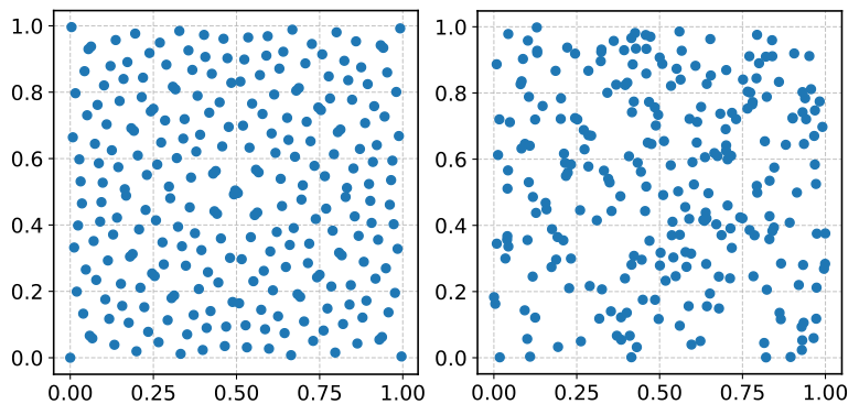
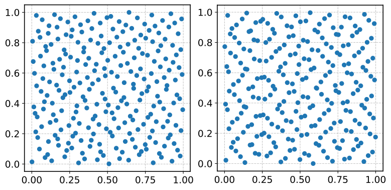
The easiest way to get acquainted with low-discrepancy sequence is maybe just look at how the compare with regular pseudo-random numbers.
import numpy as npfrom matplotlib import pyplot as pltfrom scipy.stats import qmcrng = np.random.default_rng(313)m =8n =2**mfig, (ax1, ax2) = plt.subplots(1, 2, constrained_layout=True)# Generate n points using a Sobol sequence in 2 dimensions.sampler = qmc.Sobol(d=2, scramble=False)x, y = sampler.random_base2(m).Tax1.plot(x, y, "o")ax1.set_aspect("equal")# Generate plain Monte Carlo numbers in the unit square.x = rng.uniform(size=n)y = rng.uniform(size=n)ax2.plot(x, y, "o")ax2.set_aspect("equal")
Can you guess who is who? (Yes: left is a Sobol sequence, right is the usual PRNG.) A quick look at the two plots should make you jump on your chair and scream: ah ah—now I can see where the variance reduction comes from!
Warning
As most QMC constructions, Sobol sequences are designed to generate samples of special sizes—in this case a power of \(2\). Generating \(100\) numbers might get you a less accurate estimate for an integral than generating \(64\). Make sure you read the fine prints in the Scipy documentation.
How do we get the machinery to work for our purposes? Easier done than said.
import numpy as npfrom scipy.stats import qmcdef sobol_integral(func, a, b, m):"""Calculate the definite integral of a function by means of the sample mean method using a one-dimensional Sobol sequence. Arguments --------- func : callable The integrand f(x). It must accept a NumPy array as the only argument and return an array of function values with the same shape. a : float Lower bound of the integration interval. b : float Upper bound of the integration interval (must be > a). m : int The power of 2 defining the number of points in the sequence (n = 2**m). Returns ------- I : float Estimate of the integral. """ sampler = qmc.Sobol(d=1, scramble=False) x = sampler.random_base2(m) x = qmc.scale(x, a, b)return np.mean(func(x))def f(x):return1./ (1.+ x**2.)I = sobol_integral(f, 0., 1., m=10)target = np.pi /4.print(f"Sobol sequence: relative error = {abs(I - target) / target:.1e}")
Sobol sequence: relative error = 3.1e-04
If you paid attention, you will have noticed that we are not returning an estimate for the uncertainty, here. This points out to a very fundamental fact: Sobol sequences are strictly deterministic—if you don’t do anything specific they really behave as a regular grid.
Since the values in the sequence are not statistically independent (nor they are designed to look as if they were), you cannot use your statistics textbook to attach an uncertainty to the estimate starting from the first principles, as we did with the Monte Carlo methods.
And this is where the scramble arguments comes into play. If you set it to True (which, by the way, is its default value) two things happen:
the resulting points are randomized;
you get different values every time.
from scipy.stats import qmcm =3sampler1 = qmc.Sobol(d=1)sampler2 = qmc.Sobol(d=1)print(sampler1.random_base2(m).T)print(sampler2.random_base2(m).T)
And yet, all of this happens preserving the low-discrepancy structure of the sequence, so you get all the good properties the thing was defined for, but now you can take the variation across a number of independently scrambled sequences to estimate the uncertainty in you calculation.
import numpy as npfrom matplotlib import pyplot as pltfrom scipy.stats import qmcrng = np.random.default_rng(313)m =8n =2**mfig, (ax1, ax2) = plt.subplots(1, 2, constrained_layout=True)sampler1 = qmc.Sobol(d=2, scramble=True)x, y = sampler1.random_base2(m).Tax1.plot(x, y, "o")ax1.set_aspect("equal")sampler2 = qmc.Sobol(d=2, scramble=True)x, y = sampler2.random_base2(m).Tax2.plot(x, y, "o")ax2.set_aspect("equal")
The typical convergence rate for a well-behaved QMC integral is far better that the PRNG counterpart, \[
\frac{\sigma_I}{\hat{I}} \propto n^{-1}.
\]
3.6 Executive summary
When integrating a one-dimensional function, classical quadrature methods such as the ones provided by scipy.quad() are hard to beat—yes, you can find counter-examples to this, but you really have to look hard for them.
As the dimensionality of you problem grows, Monte Carlo and QMC techniques become an attractive alternative, as the convergence rate remain constant. For the purpose of integration, Monte Carlo methods are limited to a convergence rate of \(n^{-\frac{1}{2}}\), while QMC typically achieves a much better rate of \(n^{-1}\) (or even better, in some situations) and is therefore to be preferred.
This all said, there are cases (and many, too) where you really want sequences whose elements look statistically independent from each other, and that is precisely what we shall start exploring in the next section.
Joe, Stephen, and Frances Y. Kuo. 2008. “Constructing Sobol Sequences with Better Two-Dimensional Projections.”SIAM Journal on Scientific Computing 30 (5): 2635–54. https://doi.org/10.1137/070709359.
Sobol’, I. M. 1967. “On the Distribution of Points in a Cube and the Approximate Evaluation of Integrals.”Zhurnal Vychislitel’noi Matematiki i Matematicheskoi Fiziki 7 (4): 784–802.